Generative Adversarial Networks (GANs): From Theory to Real-World Applications
Meta Description: Master Generative Adversarial Networks (GANs) theory and applications. Learn architecture, training strategies, StyleGAN, diffusion models, and practical implementation for image generation.
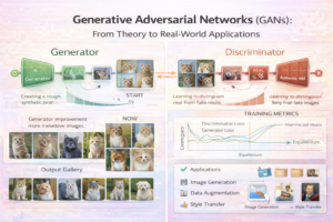
Introduction: The Power of Adversarial Generation
Generative Adversarial Networks, introduced by Ian Goodfellow in 2014, represent one of the most creative paradigms in deep learning. Instead of directly learning to generate images, two networks compete: a Generator creates fake images, while a Discriminator tries to detect them. This adversarial process produces remarkably realistic outputs.
By 2026, GANs have evolved dramatically. StyleGAN produces nearly photorealistic faces, Diffusion Models often outperform GANs, and GANs remain essential for image editing, super-resolution, and style transfer. This guide covers GAN theory, practical training, and real-world applications.
Core GAN Concept: The Adversarial Game
The Setup
Two networks compete in a game:
- Generator (G): Takes random noise z, produces fake image G(z)
- Discriminator (D): Classifies whether input is real (from dataset) or fake (from G)
The Objective Function (Minimax Game)
min_G max_D E[log D(x)] + E[log(1 - D(G(z)))]
Where:
- x = real image from dataset
- z = random noise
- D(x) = probability discriminator thinks x is real
- D(G(z)) = probability discriminator thinks fake image is real
Game Dynamics:
- Discriminator wants: D(x) → 1 (recognize real), D(G(z)) → 0 (reject fake)
- Generator wants: D(G(z)) → 1 (fool discriminator)
- Equilibrium: D(x) = D(G(z)) = 0.5 (discriminator can’t distinguish)
Training Process
for each training iteration:
 1. Sample real batch {x_1, ..., x_m} from dataset
 2. Sample noise {z_1, ..., z_m}
 3. Generate fake batch {G(z_1), ..., G(z_m)}
4. Update Discriminator:
loss_D = -log(D(x)) - log(1 - D(G(z)))
Backprop, gradient step
5. Update Generator:
loss_G = -log(D(G(z))) // Generator wants to fool D
Backprop, gradient step
Key Insight: Generator never sees real images directly. It learns to generate through discriminator feedback only.
GAN Training Challenges
Challenge 1: Mode Collapse
Generator learns to produce only a few types of images, ignoring diversity.
Symptom: Generated dataset contains only faces of same person, or all same pose/emotion.
Cause: Generator finds one “easy” pattern that fools discriminator, doesn’t improve.
Solutions:
- Minibatch Discrimination: Discriminator looks at entire batch, penalizes if batch lacks diversity
- Spectral Normalization: Constrain discriminator to be Lipschitz continuous (smooth)
- Experience Replay: Discriminator trains on mix of recent and old fake images
- Multiple Loss Terms: Add diversity loss to generator objective
Challenge 2: Non-Convergence and Instability
Loss oscillates wildly, training collapses.
Causes:
- Discriminator gets too strong, provides useless gradients
- Generator loss vanishes (log becomes saturated)
- Training hyperparameters mismatched
Solutions (Wasserstein GAN):
- Change Loss: Use Wasserstein distance instead of JS divergence
- New Objective: min_G max_D E[D(x)] – E[D(G(z))]
- Benefit: Provides meaningful gradient even when distributions don’t overlap
- Result: Much more stable training
Challenge 3: Low Resolution and Blurry Images
Especially earlier GAN architectures produce 64×64 or lower resolution images.
Solution: Progressive Growing
- Start training with low resolution (4×4)
- Gradually add layers, increase resolution
- 4×4 → 8×8 → 16×16 → 32×32 → 64×64 → 128×128 → 256×256 → 512×512
- Each stage trains until convergence
- Result: Able to generate 1024×1024+ resolution images
Evolution of GAN Architectures
DCGAN (2016) – Convolutional GANs
First successful architecture using convolutional layers.
- Generator: Transposed convolutions (fractional-stride convolutions) to upsample
- Discriminator: Standard convolutions to downsample
- Key Innovation: Batch normalization in both networks
- Results: 64×64 images of decent quality
- Significance: Practical architecture that actually works
Pix2Pix (2017) – Conditional GANs
Generate images conditioned on input (e.g., sketch → photo).
- Generator: Takes image as input (not just noise) → U-Net architecture
- Loss: Adversarial loss + L1 reconstruction loss
- Results: High-quality paired image translation
- Applications: Sketch to photo, semantic map to street scene, day to night
StyleGAN (2019) – Style Control
Separate content (high-level features) from style (low-level details).
- Generator Architecture: Constant 4×4 input + style modulation at each layer
- Style Mixing: Use different style codes for different resolutions
- Results: Nearly photorealistic faces, precise control over style
- Key Metrics: FID score 4.40 (human-level quality)
- Applications: Face generation, style transfer, image editing
StyleGAN2 & StyleGAN3
- StyleGAN2: Improved convergence, artifact removal
- StyleGAN3: Equivariant generation (respects transformations like rotation)
- Current Quality: Indistinguishable from real photos at 1024×1024
CycleGAN (2017) – Unpaired Image Translation
Translate images between domains without paired training data.
- Key Idea: Use cycle consistency loss: X → Y → X should recover X
- Applications: Photo ↔ painting, horse ↔ zebra, summer ↔ winter
- Advantage: No need for paired training data
- Quality: Decent but not as good as pix2pix (because unpaired)
Diffusion Models vs GANs (2020+)
Diffusion models (DALL-E and text-to-image tools, Stable Diffusion, Midjourney) now often outperform GANs.
| Aspect | GANs | Diffusion Models |
|---|---|---|
| Image Quality | Excellent (StyleGAN: FID 4.4) | Excellent (Stable Diffusion: FID 7.8) |
| Training Stability | Difficult, requires tuning | Stable, straightforward training |
| Mode Coverage | Can mode collapse | Better coverage of distribution |
| Inference Speed | Fast (single forward pass) | Slow (many denoising steps) |
| Conditional Generation | Requires retraining for conditions | Easy (classifier-free guidance) |
| Current Dominance | Niche applications | State-of-the-art (DALL-E 3, Midjourney) |
Real-World GAN Applications
Application 1: Face Generation and Synthesis
Use Case: Generate diverse human faces for avatars, testing, privacy.
Technology: StyleGAN3 or similar
Results:
- Quality: Photorealistic at 1024×1024
- Control: Adjust age, gender, expression via latent space
- Cost: Single GPU fine-tuning (~$500)
- Application Example: Synthetic avatars for online platforms (avoid privacy issues)
Application 2: Image Super-Resolution
Use Case: Enhance low-resolution images to high-resolution.
Technology: SRGAN (Super-Resolution GAN) or RealESRGAN
Results:
- 4x upsampling: 512×512 → 2048×2048
- PSNR improvement: ~3-5 dB
- Perceptual quality: Much better than traditional interpolation
- Inference: 1-2 seconds per image
Real Example:
- Input: Low-res photo from old camera
- Output: High-res version with recovered details
- Cost: ~$0.01 per image on cloud service
Application 3: Image-to-Image Translation
Use Case: Convert image from one domain to another (sketch to photo, day to night).
Technology: Pix2Pix for paired data, CycleGAN for unpaired
Real Examples:
- Architectural Sketch → Photo: Architects visualize designs
- Grayscale → Colorization: Colorize old photos
- Semantic Map → Street Scene: Generate realistic street scenes from semantic segmentation
- Season Transfer: Convert summer photo to winter
Cost & Speed:
- Training: 2-4 days on 1 GPU with 1K-10K paired images
- Inference: 50-200ms per image
- Accuracy: 80-90% similarity to real domain
Application 4: Data Augmentation
Use Case: Generate synthetic training data when real data is scarce.
Scenario: Medical AI needs 5,000 training images but only 500 real images available.
Solution: Train GAN on 500 images, generate 4,500 synthetic images
Results:
- Model trained on real + synthetic data achieves 88% accuracy
- Model trained on real-only achieves 76% accuracy
- Improvement: 12 percentage points
- Cost: $500-2,000 to train GAN
Caution: Synthetic data quality must be high. Poor-quality synthetic data hurts accuracy more than helps.
Application 5: Style Transfer
Use Case: Apply artistic style to photos (Van Gogh style, specific artist, brand aesthetic).
Technology: AdaIN-based or style-transfer networks
Results:
- Content preserved while style applied
- Inference: <1 second per image
- Highly controllable (blend amount, style strength)
Commercial Examples:
- Prisma app: Real-time artistic style transfer
- Deep Dream: Psychedelic dream-like transformations
- Brand applications: Convert product photos to brand aesthetic
Application 6: Video Generation and Frame Interpolation
Use Case: Generate smooth video from few frames, interpolate between frames.
Technology: Temporal GANs, MoCoGAN, DVD-GAN
Current State (2026):
- Frame interpolation: Excellent (240fps from 30fps video)
- Video generation from noise: Still challenging, lower quality
- Video generation from text: Emerging (Sora, Runway Gen-3)
Results:
- PSNR: 25-30 dB for interpolation
- Latency: 100-500ms per frame
- Resolution: Up to 1080p
GAN Implementation Practical Guide
Building a Simple DCGAN from Scratch
import torch
 import torch.nn as nn
class Generator(nn.Module):
def __init__(self, z_dim=100):
super().__init__()
self.model = nn.Sequential(
nn.ConvTranspose2d(z_dim, 512, 4, 1, 0),
nn.BatchNorm2d(512),
nn.ReLU(),
nn.ConvTranspose2d(512, 256, 4, 2, 1),
nn.BatchNorm2d(256),
nn.ReLU(),
nn.ConvTranspose2d(256, 128, 4, 2, 1),
nn.BatchNorm2d(128),
nn.ReLU(),
nn.ConvTranspose2d(128, 3, 4, 2, 1),
nn.Tanh()
)
def forward(self, z):
return self.model(z)
class Discriminator(nn.Module):
def __init__(self):
super().__init__()
self.model = nn.Sequential(
nn.Conv2d(3, 64, 4, 2, 1),
nn.LeakyReLU(0.2),
nn.Conv2d(64, 128, 4, 2, 1),
nn.BatchNorm2d(128),
nn.LeakyReLU(0.2),
nn.Conv2d(128, 256, 4, 2, 1),
nn.BatchNorm2d(256),
nn.LeakyReLU(0.2),
nn.Conv2d(256, 1, 4, 1, 0),
nn.Sigmoid()
)
def forward(self, x):
return self.model(x)
# Training loop
gen = Generator()
disc = Discriminator()
opt_g = torch.optim.Adam(gen.parameters(), lr=0.0002)
opt_d = torch.optim.Adam(disc.parameters(), lr=0.0002)
criterion = nn.BCELoss()
for epoch in range(100):
for real_images, _ in dataloader:
batch_size = real_images.size(0)
# Update Discriminator
real_labels = torch.ones(batch_size, 1)
fake_labels = torch.zeros(batch_size, 1)
z = torch.randn(batch_size, 100)
fake_images = gen(z)
d_loss_real = criterion(disc(real_images), real_labels)
d_loss_fake = criterion(disc(fake_images.detach()), fake_labels)
d_loss = d_loss_real + d_loss_fake
opt_d.zero_grad()
d_loss.backward()
opt_d.step()
# Update Generator
z = torch.randn(batch_size, 100)
fake_images = gen(z)
g_loss = criterion(disc(fake_images), real_labels)
opt_g.zero_grad()
g_loss.backward()
opt_g.step()
Training Tips
- Use Spectral Normalization: Stabilizes discriminator, reduces mode collapse
- Separate Learning Rates: Discriminator often needs higher learning rate
- Monitor FID Score: Frechet Inception Distance measures quality (lower is better, <10 is good)
- Avoid Batch Size Too Small: Minimum 32-64
- Use Gradient Penalty: Prevents discriminator from becoming too strong
- Checkpoint Regularly: Save generator/discriminator states frequently
Evaluation Metrics
FID (Fréchet Inception Distance)
- Measures distance between real and fake image distributions
- Lower is better. 100 is poor
- Based on feature statistics from pre-trained Inception network
- Standard metric for GAN evaluation
Inception Score (IS)
- Measures image quality and diversity
- Higher is better. >8 is good, >15 is excellent
- Less reliable than FID (can be gamed)
Human Evaluation
- Gold standard: have humans rate image quality (1-10 scale)
- Percentage fooled: how many humans think fake image is real
- Time consuming but most reliable
Key Takeaways
- GANs are powerful but challenging: Training is unstable compared to supervised learning. Requires careful tuning and architecture selection.
- Diffusion models often better now: For general image generation, diffusion models (DALL-E 3, Stable Diffusion) often outperform GANs in quality and training stability.
- StyleGAN for faces: For high-quality face generation, StyleGAN3 is still unmatched. Achieves photorealism at 1024×1024.
- Mode collapse is manageable: With spectral normalization, gradient penalty, and minibatch discrimination, mode collapse is largely preventable.
- Conditional GANs are practical: Pix2Pix and CycleGAN enable practical applications like image translation and super-resolution.
- Data requirements matter: Need at least 1,000 images of target distribution. More is better. Mode collapse more likely with small datasets.
- Inference is fast: Single forward pass, unlike diffusion (many denoising steps). Good for real-time applications.
- Evaluation is non-obvious: No standard metric. Use FID for diversity, IS for quality, human evaluation for ultimate judgment.
Getting Started
Start with a pre-trained StyleGAN3 for face generation (most polished). If you need custom domain (medical images, products), train DCGAN with Spectral Normalization on your data (1-2 weeks on single GPU). Monitor FID score to track progress. If you need image translation, use CycleGAN (no paired data needed). For most new applications, first check if diffusion models work better—they often do.
Continue Learning: Related Articles
Transformer Architecture: The Technology Powering Modern AI
The Transformer Revolution in AI
In 2017, a groundbreaking paper titled "Attention is All You Need" introduced the Tr…
📖 5 min read
Understanding Neural Networks: A Comprehensive Guide for Beginners
Introduction to Neural Networks
Neural networks are the backbone of modern artificial intelligence and deep learning….
📖 4 min read
Recurrent Neural Networks (RNN) vs Transformers: Which Should You Choose for Sequential Data?
Recurrent Neural Networks (RNN) vs Transformers: Which Should You Choose for Sequential Data?
Meta Description: Compare…
📖 11 min read
Convolutional Neural Networks: Complete Architecture Guide from Basic to Advanced
Convolutional Neural Networks: Complete Architecture Guide from Basic to Advanced
Meta Description: Master CNN architec…
📖 10 min read
💡 Explore 80+ AI implementation guides on Harshith.org