Convolutional Neural Networks: Complete Architecture Guide from Basic to Advanced
Introduction: Why CNNs Dominate Vision
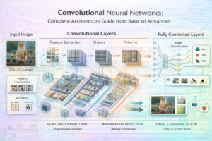
Convolutional Neural Networks (CNNs) revolutionized computer vision. Unlike fully-connected networks, CNNs exploit the spatial structure of images, learning hierarchical features: low-level edges in early layers, middle-level shapes in middle layers, and high-level objects in deeper layers.
Since AlexNet’s landmark 2012 ImageNet victory, CNNs have advanced dramatically. Modern architectures like ResNet, EfficientNet, and Vision Transformers achieve superhuman accuracy on many vision tasks. This comprehensive guide takes you from understanding convolution operations to implementing state-of-the-art architectures.
Fundamental Building Blocks
The Convolution Operation
A convolution applies a small filter (kernel) across the image, computing dot products at each position.
- Filter Size (Kernel): Typically 3×3, 5×5, or 7×7. Larger filters capture larger features.
- Stride: How many pixels the filter moves each step. Stride=1: move 1 pixel. Stride=2: move 2 pixels (reduces spatial dimensions).
- Padding: Add border pixels to preserve spatial dimensions. “Same” padding preserves size, “valid” padding doesn’t.
- Channels: Number of filters applied. Each filter learns different features (edges, corners, textures).
Convolution Mathematics:
output[i,j] = sum(input[i+a, j+b] * kernel[a,b] for a,b in kernel_range) + bias
Example: A 3×3 filter scanning a 32×32 image with stride=1 and no padding produces a 30×30 output.
Pooling: Dimensionality Reduction
Reduces spatial dimensions, increases computational efficiency, and provides translation invariance.
- Max Pooling: Keep maximum value in each window (2×2 typical). Preserves most important features.
- Average Pooling: Take average in each window. Smoother, less prone to overfitting.
- Global Average Pooling: Average entire feature map to single value. Used at end of networks.
Effect: 2×2 max pooling with stride=2 reduces 32×32 to 16×16 (4x fewer parameters).
Activation Functions
ReLU (Rectified Linear Unit): max(0, x)
- Most common activation (simple, fast, effective)
- Sparse activations (50% outputs are 0)
- Problem: Dying ReLU (neurons output 0 forever)
Leaky ReLU: max(0.01*x, x)
- Addresses dying ReLU problem
- Always has gradient
- Slightly better performance in practice
GELU (Gaussian Error Linear Unit): x * Φ(x)
- Modern activation, smooth unlike ReLU
- Used in Vision Transformers
- Slightly slower to compute
Batch Normalization
Normalize activations so mean=0, std=1 within each batch. Revolutionary technique introduced in 2015.
- Allows higher learning rates
- Reduces internal covariate shift
- Acts as regularizer (reduces overfitting)
- Typical improvement: 2-5% accuracy
Mathematical Definition:
y = gamma * (x - batch_mean) / sqrt(batch_var + epsilon) + beta
Where gamma and beta are learnable parameters.
Classic CNN Architectures
LeNet (1998) – The Foundation
First successful CNN for handwritten digit recognition (MNIST).
- Architecture: Conv → ReLU → MaxPool → Conv → ReLU → MaxPool → Fully Connected → Output
- Parameters: ~60K
- Accuracy (MNIST): 99.2%
- Significance: Proved convolution’s effectiveness
- Historical Note: Yann LeCun used this for checking bank checks in 1990s
AlexNet (2012) – Modern Deep Learning’s Birth
Won ImageNet 2012 with 15.3% top-5 error (much better than previous 26%). Launched deep learning revolution.
- Architecture: 8 layers (5 convolutional + 3 fully connected)
- Key Innovations: ReLU activation, Dropout for regularization, GPU acceleration
- Parameters: 60M
- ImageNet Accuracy: 84.7% top-1
- Impact: Sparked explosion of deep learning research
VGG (2014) – Simplicity and Depth
Demonstrated that network depth matters. Simple architecture: stacked 3×3 convolutions.
- Architecture: All filters 3×3, gradually increase channels (64 → 128 → 256 → 512)
- Depth Variants: VGG16 and VGG19 (number = total layers)
- Parameters: 138M (VGG16)
- ImageNet Accuracy: 87.3% top-1 (VGG16)
- Key Insight: Several small filters (3×3) equivalent to larger filter but more parameters efficient and better regularization
- Disadvantage: Massive parameter count, slow training
GoogLeNet/Inception (2014) – Multi-Scale Feature Learning
Introduced Inception modules: parallel convolutions of different sizes.
- Key Innovation: 1×1 convolutions to reduce dimensionality (bottleneck)
- Architecture: Multiple 1×1, 3×3, 5×5, pooling in parallel
- Parameters: 12M (4x fewer than VGG)
- ImageNet Accuracy: 89.5% top-1
- Advantage: Better parameter efficiency than VGG
ResNet (2015) – Skip Connections Transform Deep Learning
Revolutionized deep neural networks by solving vanishing gradient problem with skip connections.
Key Innovation: Residual Block
output = x + F(x) # Add input to output of layers
Instead of learning y = F(x), learn y = x + F(x). This is equivalent to learning the residual (difference).
- Benefits: Gradients flow directly through skip connections, allows training very deep networks (152 layers)
- Architecture Variants: ResNet18, ResNet34, ResNet50, ResNet101, ResNet152
- Bottleneck Design: ResNet uses 1×1 → 3×3 → 1×1 to reduce parameters
- ImageNet Accuracy: 92.1% top-1 (ResNet152)
- Parameters: 60M (ResNet50)
- Impact: Enabled training networks 10x deeper than previously possible
DenseNet (2017) – Dense Connections
Connect each layer to all previous layers (not just immediate predecessor).
- Key Idea: Concatenate all previous features (not sum like ResNet)
- Parameters: 7M (DenseNet121) – much more efficient than ResNet
- ImageNet Accuracy: 90.2% (DenseNet121)
- Advantages: Better gradient flow, feature reuse, regularization effect
- Disadvantage: Higher memory during training due to concatenation
Modern Efficient Architectures
MobileNet (2017) – Efficient Mobile Inference
Designed for mobile/embedded devices. Uses depthwise separable convolutions.
- Key Technique: Depthwise Separable Convolution = Depthwise (per-channel) + Pointwise (1×1) convolution
- Parameter Reduction: 8-9x fewer parameters than standard convolutions
- Accuracy/Parameters Trade-off: 88% (MobileNetV1) with only 4.2M parameters
- Inference Speed: 22 FPS on mobile GPU, <100ms latency
- Variants: MobileNetV2 (2018), MobileNetV3 (2019)
EfficientNet (2019) – Optimal Scaling
Systematically scale network depth, width, and resolution for maximum efficiency.
- Compound Scaling Rule: α^d × β^w × γ^r = 2^φ, where depth, width, resolution scale proportionally
- Variants: EfficientNet-B0 to B7 (progressively larger)
- Performance Comparison:
| Model | Top-1 Accuracy | Parameters | FLOPs |
|---|---|---|---|
| EfficientNet-B0 | 77.0% | 5.3M | 0.4B |
| EfficientNet-B4 | 83.5% | 19.3M | 4.2B |
| EfficientNet-B7 | 84.5% | 66.3M | 37B |
| ResNet50 | 76.5% | 25.6M | 4.1B |
Key Advantage: EfficientNet-B0 achieves 77% accuracy with 5.3M parameters (ResNet50 needs 25.6M for 76.5%)
Vision Transformers: The CNN Paradigm Shift
Vision Transformer (ViT) – 2020
Applies transformer architecture (from NLP) directly to image patches, challenging CNN dominance.
How ViT Works:
- Divide image into fixed-size patches (16×16, 32×32)
- Linearize each patch and embed (project to d dimensions)
- Add position embeddings
- Pass through transformer layers (multi-head attention + MLP)
- Use [CLS] token output for classification
Advantages Over CNNs:
- Global receptive field from start (attention can relate distant pixels)
- Theoretically more powerful (can learn any permutation of pixels)
- Better scaling (performance improves with more data/compute)
- Transfer learning advantages (pre-train on massive datasets)
Disadvantages:
- Requires large datasets to train from scratch (≥10M images)
- Slower inference than CNNs
- No built-in inductive bias about images (CNNs assume spatial locality)
Vision Transformer Variants:
| Model | Resolution | Top-1 Accuracy (ImageNet-21K) | Parameters | Best For |
|---|---|---|---|---|
| ViT-Tiny | 224×224 | 72.3% | 5.7M | Mobile/edge, requires fine-tuning |
| ViT-Small | 224×224 | 79.9% | 22M | Medium compute, good accuracy |
| ViT-Base | 224×224 | 84.2% | 86M | Standard choice, SOTA accuracy |
| ViT-Large | 224×224 | 86.9% | 307M | Maximum accuracy, high compute needed |
Practical Comparison: When to Use ViT vs CNN
- Use CNN when: Limited data (<10K images), need inference speed (<50ms), mobile deployment, constrained compute
- Use ViT when: Abundant data (100K+ images), accuracy paramount, can afford higher latency (100-200ms), training compute available
- Practical recommendation: Start with ResNet or EfficientNet. Switch to ViT if accuracy stalls.
Advanced Architecture Techniques
Attention Mechanisms in CNNs
Add attention layers to focus on important regions.
Channel Attention: Learn to weight different feature channels
channel_weights = sigmoid(FC2(ReLU(FC1(global_avg_pool(x)))))
 output = x * channel_weights
Spatial Attention: Learn to weight different spatial regions
spatial_weights = sigmoid(Conv1x1(concat(max_pool(x), avg_pool(x))))
 output = x * spatial_weights
Effect: Typically improves accuracy by 1-3%
Multi-Scale Feature Fusion
Combine features at different resolutions (large receptive field captures context, small captures detail).
- Feature Pyramid Networks (FPN): Build multi-scale feature maps
- Path Aggregation Networks (PAN): Improve information flow between scales
- Bidirectional FPN (BiFPN): Weighted bidirectional feature fusion
- Typical improvement: 2-5% accuracy on small object tasks
Neural Architecture Search (NAS)
Automatically discover optimal architectures instead of hand-designing.
- Process: Define search space (layer types, connections), use evolutionary algorithm or reinforcement learning to find best architecture
- Examples: EfficientNet discovered via NAS, NASNet (Google’s method)
- Results: Often find better architectures than human design
- Limitation: Very expensive (days/weeks of GPU compute)
Practical Implementation Guide
Image Classification from Scratch (Transfer Learning)
import torchvision.models as models
 import torch.nn as nn
 import torch.optim as optim
# Load pre-trained ResNet50
model = models.resnet50(pretrained=True)
# Freeze early layers (pre-trained features are good)
for param in model.layer1.parameters():
param.requires_grad = False
for param in model.layer2.parameters():
param.requires_grad = False
# Replace final layer for your task
num_classes = 10 # Your classification task
model.fc = nn.Linear(model.fc.in_features, num_classes)
# Optimization
optimizer = optim.Adam(model.parameters(), lr=1e-4)
loss_fn = nn.CrossEntropyLoss()
# Training loop
for epoch in range(10):
for images, labels in train_loader:
outputs = model(images)
loss = loss_fn(outputs, labels)
optimizer.zero_grad()
loss.backward()
optimizer.step()
Model Selection Strategy
- Start with pre-trained: Always use ImageNet pre-training (transfer learning works)
- Baseline: Start with ResNet50 (proven, fast)
- If accuracy insufficient: Try EfficientNet-B4/B5 (better efficiency-accuracy)
- If speed critical: Use MobileNet or EfficientNet-B0/B1
- If money unlimited: Try ViT-Base with massive data
Training Best Practices
- Learning Rate: Start with 1e-4 for fine-tuning (smaller than pre-training)
- Batch Size: 32-128 depending on GPU memory
- Data Augmentation: RandAugment, AutoAugment improve accuracy 2-5%
- Warm-up: Gradually increase learning rate first 5-10% of training
- Regularization: Dropout, weight decay, batch norm prevent overfitting
- Early Stopping: Monitor validation accuracy, stop if no improvement 10 epochs
Key Takeaways
- CNNs exploit spatial structure: Convolutions, pooling, and hierarchical features make them perfect for images. This inductive bias is powerful.
- Depth enables better features: ResNet proved deep networks work (with skip connections). Deeper typically means better.
- Efficiency matters: EfficientNet shows how to scale networks optimally. Modern approaches achieve same accuracy with 5-10x fewer parameters.
- Vision Transformers are powerful: ViT achieves SOTA accuracy but needs massive data and compute. CNN still better for small data.
- Transfer learning is essential: Pre-trained ImageNet weights accelerate training and improve accuracy. Always use pre-training.
- Model choice is context-dependent: ResNet for general purpose, EfficientNet for efficiency, MobileNet for mobile, ViT for maximum accuracy.
- Attention mechanisms help: Adding attention improves accuracy by 1-3% with modest computational cost.
Architecture Decision Tree
What’s your constraint?
Speed critical (<50ms)? → MobileNet or EfficientNet-B0
Mobile deployment? → MobileNet or EfficientNet-B0/B1
Balanced accuracy/speed? → ResNet50 or EfficientNet-B2/B3
Maximum accuracy, compute available? → EfficientNet-B5+ or ViT-Base
Massive dataset (1M+ images)? → ViT-Base or ViT-Large
Getting Started
Start with PyTorch torchvision models. Load ResNet50 pre-trained, fine-tune on your data. Measure accuracy and speed. If accuracy is good enough, done. If not, move to EfficientNet. Benchmark everything—model size, inference speed, and accuracy—against your requirements. Spend more time on data quality and augmentation than architecture engineering.
Continue Learning: Related Articles
Understanding Neural Networks: A Comprehensive Guide for Beginners
Introduction to Neural Networks
Neural networks are the backbone of modern artificial intelligence and deep learning….
📖 4 min read
Transformer Architecture: The Technology Powering Modern AI
The Transformer Revolution in AI
In 2017, a groundbreaking paper titled "Attention is All You Need" introduced the Tr…
📖 5 min read
Generative Adversarial Networks (GANs): From Theory to Real-World Applications
Generative Adversarial Networks (GANs): From Theory to Real-World Applications
📖 11 min read
Recurrent Neural Networks (RNN) vs Transformers: Which Should You Choose for Sequential Data?
Recurrent Neural Networks (RNN) vs Transformers: Which Should You Choose for Sequential Data?
📖 12 min read
💡 Explore 80+ AI implementation guides on Harshith.org