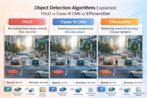
Object Detection Algorithms Explained: YOLO vs Faster R-CNN vs EfficientDet 2026
Meta Description: Compare YOLO, Faster R-CNN, and EfficientDet object detection algorithms. Learn speed, accuracy trade-offs, and which model to use for your computer vision application in 2026.
Introduction: The Object Detection Problem
Object detection is one of the most practical computer vision tasks. Real-world applications need to locate and classify multiple objects in images or video streams with minimal latency. The challenge: balancing speed and accuracy while minimizing computational requirements.
In 2026, the landscape has evolved dramatically. YOLOv8 and v11 dominate real-time applications, Faster R-CNN remains the accuracy champion, and EfficientDet provides the best speed-accuracy trade-off for resource-constrained environments. This guide explains how each works and helps you choose the right algorithm for your use case.
The Object Detection Paradigm: Two Approaches
One-Stage Detectors (YOLO, SSD, RetinaNet)
Process the entire image once, predicting bounding boxes and class probabilities simultaneously.
- Speed: 30-200 FPS depending on model size
- Accuracy: Moderate (mAP 40-55%)
- Best for: Real-time applications, embedded systems
- Latency: 5-30ms per image
Two-Stage Detectors (Faster R-CNN, Mask R-CNN, Cascade R-CNN)
First identify region proposals (where objects might be), then classify and refine bounding boxes.
- Speed: 5-30 FPS
- Accuracy: Higher (mAP 50-65%)
- Best for: Accuracy-critical applications, batch processing
- Latency: 100-300ms per image
YOLO: Real-Time Object Detection
Overview
You Only Look Once (YOLO) was introduced in 2016 and revolutionized object detection by treating it as a regression problem. Instead of finding regions first, YOLO divides the image into a grid and directly predicts bounding boxes and confidence scores.
How YOLO Works:
- Divide image into SxS grid (typically 13×13 to 19×19)
- For each grid cell, predict:
- B bounding boxes (x, y, width, height, confidence)
- Class probabilities (one per class)
- Filter predictions by confidence threshold (typically 0.5)
- Apply Non-Maximum Suppression (NMS) to remove duplicates
YOLO Versions Comparison
| Version | Release | Backbone | Speed (GPU) | mAP COCO | Parameters | Key Innovation |
|---|---|---|---|---|---|---|
| YOLOv5 | 2020 | CSPDarknet | 50 FPS | 50.7% | 27M | Data augmentation, auto-scaling |
| YOLOv6 | 2022 | EfficientRep | 60 FPS | 52.6% | 18M | Decoupled head, anchor-free |
| YOLOv7 | 2022 | ELAN | 70 FPS | 53.7% | 36M | Efficient Reparameterized model, skip connections |
| YOLOv8 | 2023 | YOLOv3 backbone | 80 FPS | 53.9% | 25M | Modular design, multi-task (detection/segmentation/pose) |
| YOLOv10 | 2024 | Improved CSP | 100 FPS | 54.3% | 20M | NMS-free post-processing |
| YOLOv11 | 2024-2025 | Optimized CSP | 120 FPS | 55.1% | 17M | Edge computing optimizations |
YOLO Advantages:
- Extremely fast (real-time on GPU, 30+ FPS on CPU)
- Excellent speed-accuracy trade-off
- Easy to use (high-level APIs available)
- Works well with data augmentation
- Simple deployment (single model, no region proposal stage)
- Supports multiple tasks (detection, segmentation, pose estimation)
YOLO Disadvantages:
- Lower accuracy than two-stage detectors (especially on small objects)
- Struggles with multiple small objects in same grid cell
- Requires precise localization in grid cell (can miss objects at cell boundaries)
- Less robust to unusual aspect ratios
YOLO Implementation Example:
from ultralytics import YOLO
# Load pre-trained model
model = YOLO('yolov8n.pt')
# Inference
results = model('image.jpg')
# Results
for result in results:
boxes = result.boxes
for box in boxes:
x1, y1, x2, y2 = box.xyxy[0]
confidence = box.conf[0]
class_id = box.cls[0]
print(f"Box: ({x1}, {y1}, {x2}, {y2}), Confidence: {confidence:.2f}, Class: {class_id}")
Faster R-CNN: The Accuracy Champion
Overview
Faster Region-Based Convolutional Neural Network (Faster R-CNN) is the state-of-the-art two-stage detector introduced in 2015. It finds region proposals first (where objects likely exist), then refines these proposals with classification.
How Faster R-CNN Works:
- Backbone: Extract features from image (ResNet, EfficientNet, etc.)
- Region Proposal Network (RPN): Generates candidate regions that might contain objects
- Region of Interest Pooling (RoI Pool): Extracts fixed-size features for each proposal
- Classification and Bounding Box Regression: Classifies each region and refines boxes
Faster R-CNN Architecture Variants
| Architecture | Backbone | Speed | mAP COCO | Parameters | Best For |
|---|---|---|---|---|---|
| Faster R-CNN (ResNet-50) | ResNet-50 | 10 FPS | 58.5% | 134M | General purpose, good balance |
| Faster R-CNN (ResNet-101) | ResNet-101 | 8 FPS | 59.6% | 208M | Maximum accuracy, larger objects |
| Mask R-CNN | ResNet-50 | 8 FPS | 58.5% (detection) + segmentation | 158M | Instance segmentation, detailed object boundaries |
| Cascade R-CNN | ResNet-50 | 6 FPS | 62.1% | 140M | Ultra-high accuracy, multi-stage refinement |
| Faster R-CNN (EfficientNet-B4) | EfficientNet-B4 | 12 FPS | 59.8% | 76M | Accuracy with lower memory |
Faster R-CNN Advantages:
- Highest accuracy among traditional detectors (mAP 58-62%)
- Excellent at detecting small objects
- Two-stage approach reduces false positives
- Works well with various backbones (ResNet, EfficientNet, Vision Transformer)
- Provides confidence scores for each detection
- Highly customizable through backbone selection
Faster R-CNN Disadvantages:
- Slow (8-15 FPS on GPU, <1 FPS on CPU)
- Two-stage processing increases complexity
- High memory requirements (250MB-1GB model size)
- Slower inference not suitable for real-time video
- Harder to optimize for edge devices
Faster R-CNN Implementation:
import torchvision
 from torchvision.models.detection import fasterrcnn_resnet50_fpn
# Load pre-trained model
model = fasterrcnn_resnet50_fpn(pretrained=True)
model.eval()
# Inference
import torch
from torchvision.transforms import functional as F
image = F.to_tensor(image_pil)
predictions = model([image])
# Process results
boxes = predictions[0]['boxes']
scores = predictions[0]['scores']
labels = predictions[0]['labels']
# Filter by confidence threshold
threshold = 0.5
keep = scores > threshold
boxes = boxes[keep]
scores = scores[keep]
labels = labels[keep]
EfficientDet: Best Speed-Accuracy Trade-off
Overview
EfficientDet combines the efficiency of one-stage detectors with improved accuracy through EfficientNet backbones and a BiFPN (Bidirectional Feature Pyramid Network). Introduced by Google in 2020, it provides excellent performance across different scales.
How EfficientDet Works:
- EfficientNet Backbone: Efficient feature extraction
- BiFPN: Multi-scale feature fusion with bidirectional connections
- Detection Head: Anchor-based detection head for bounding boxes and class predictions
- Compound Scaling: Uniform scaling of depth, width, and resolution
EfficientDet Versions
| Model | Resolution | Speed (GPU) | mAP COCO | Parameters | Model Size | Use Case |
|---|---|---|---|---|---|---|
| EfficientDet-D0 | 512×512 | 97 FPS | 33.6% | 3.9M | 16MB | Mobile, edge devices, ultra-fast |
| EfficientDet-D1 | 640×640 | 73 FPS | 39.2% | 6.6M | 27MB | Edge devices, real-time video |
| EfficientDet-D2 | 768×768 | 56 FPS | 43.0% | 8.1M | 33MB | Good balance for embedded systems |
| EfficientDet-D3 | 896×896 | 37 FPS | 47.5% | 12M | 50MB | Recommended for most applications |
| EfficientDet-D4 | 1024×1024 | 20 FPS | 49.4% | 20.7M | 85MB | High accuracy + reasonable speed |
| EfficientDet-D5 | 1280×1280 | 12 FPS | 50.7% | 33.7M | 138MB | Maximum accuracy |
EfficientDet Advantages:
- Best speed-accuracy trade-off for most use cases
- Excellent accuracy-to-model-size ratio
- Lightweight models suitable for mobile/edge
- Scales uniformly from ultra-small to large models
- Good performance on small objects
- Moderate computational requirements
- Multiple model sizes for different constraints
EfficientDet Disadvantages:
- Not as fast as YOLOv8 for real-time (lower FPS)
- Not as accurate as Faster R-CNN (especially on very small objects)
- Anchor-based approach (less flexible than newer anchor-free methods)
- Fewer public implementations than YOLO
- Smaller ecosystem and community support
EfficientDet Implementation:
import tensorflow as tf
 from efficientdet import EfficientDet
# Load model
model = EfficientDet(name='efficientdet-d3', pretrained=True)
# Prepare image
image = tf.image.decode_jpeg(image_data)
image = tf.image.resize(image, [896, 896])
image = tf.expand_dims(image, 0)
# Inference
boxes, scores, classes = model(image)
# Process results
threshold = 0.5
keep = scores[0] > threshold
boxes = boxes[0][keep]
scores = scores[0][keep]
classes = classes[0][keep]
Comparative Performance Analysis
Speed Comparison (8GB GPU):
| Model | Image Size | FPS (GPU) | ms per Image | FPS (CPU) | Memory Usage |
|---|---|---|---|---|---|
| YOLOv11n | 640×640 | 120 | 8.3 | 25 | 2GB |
| YOLOv8n | 640×640 | 110 | 9.1 | 22 | 2GB |
| YOLOv8m | 640×640 | 80 | 12.5 | 12 | 4GB |
| EfficientDet-D3 | 896×896 | 37 | 27 | 3 | 3GB |
| Faster R-CNN (ResNet-50) | 800×800 | 10 | 100 | 0.3 | 6GB |
| Cascade R-CNN | 800×800 | 6 | 167 | 0.1 | 8GB |
Accuracy Comparison (COCO Dataset):
| Model | AP (Average Precision) | AP Small Objects | AP Medium Objects | AP Large Objects |
|---|---|---|---|---|
| YOLOv11 | 55.1% | 35.3% | 58.2% | 72.1% |
| YOLOv8m | 53.9% | 33.8% | 56.9% | 70.8% |
| EfficientDet-D4 | 49.4% | 30.2% | 53.1% | 66.5% |
| Faster R-CNN (ResNet-50) | 58.5% | 42.1% | 62.3% | 71.2% |
| Cascade R-CNN | 62.1% | 44.9% | 65.8% | 73.5% |
Real-World Use Case Analysis
Use Case 1: Autonomous Vehicles
Requirements: High accuracy (98%+), low latency (<50ms), robust to edge cases, detects small objects (pedestrians, cyclists)
Best Choice: Faster R-CNN with ResNet-101 + Cascade refinement
- Highest accuracy on pedestrians and small objects
- Latency acceptable for autonomous driving
- Trade-off: Higher computational cost manageable on vehicle hardware
- Typical setup: NVIDIA Orin (200 TFLOPS) running at 15-20 FPS
Use Case 2: Retail Store Inventory Tracking
Requirements: Real-time detection from multiple camera feeds, moderate accuracy (85%), edge deployment, cost-effective
Best Choice: YOLOv8m or YOLOv11n
- 70+ FPS on GPU allows real-time processing
- Accuracy sufficient for product detection
- Easy deployment via Jetson or local GPU server
- Cost: ~$2,000 one-time hardware + $0 software
Use Case 3: Mobile App (Object Detection on Smartphone)
Requirements: Ultra-low latency (<100ms), minimal memory footprint (<50MB), runs on phone CPU/GPU, good accuracy (70%+)
Best Choice: EfficientDet-D0/D1 or YOLOv8n quantized
- EfficientDet-D0: 3.9M parameters, 16MB model size, 30+ FPS on mobile GPU
- YOLOv8n quantized: 2.7M parameters, 8MB model size, 25+ FPS on mobile CPU
- Deployment via TensorFlow Lite or ONNX Runtime
- Minimal impact on battery life and storage
Use Case 4: Medical Image Analysis (X-Ray Abnormality Detection)
Requirements: Maximum accuracy (95%+), slower inference acceptable, precise localization of anomalies
Best Choice: Cascade R-CNN or Faster R-CNN with EfficientNet backbone
- Accuracy critical in medical applications
- Slower speed acceptable (batch processing overnight is fine)
- Two-stage refinement beneficial for precise localization
- Confidence scores help radiologists prioritize
Use Case 5: Video Surveillance (Multi-Object Tracking)
Requirements: Continuous real-time operation (24/7), detect people/vehicles, decent accuracy (80%), low power consumption
Best Choice: YOLOv8m with custom tracker (DeepSORT or ByteTrack)
- Fast enough for 30 FPS video at 1080p resolution
- Multi-object tracking framework available
- Power-efficient on NVIDIA Jetson Xavier (10W to 25W)
- Cost: $300 Jetson + $0 software
Practical Implementation Considerations
Model Quantization for Efficiency
All three models can be quantized (8-bit or 4-bit) to reduce inference time and model size:
- YOLO Quantization: 40-50% speed improvement with <1% accuracy drop
- EfficientDet Quantization: 50-60% speed improvement, minimal accuracy loss
- Faster R-CNN Quantization: 30-40% speed improvement, may need fine-tuning
Batch Processing for Throughput
For non-real-time applications, batch processing increases throughput:
- Process 32 images at once instead of 1
- Increases throughput by 4-8x with similar latency per batch
- Use case: analyzing security footage, content moderation, inventory counts
Ensemble Methods
Combine multiple models for maximum accuracy:
- Run YOLOv8 + Faster R-CNN, average predictions
- Typical accuracy gain: 2-4%
- Latency: Sum of both models (YOLOv8 + Faster R-CNN = ~110ms)
Model Selection Decision Tree
Start by answering:
1. Is latency critical (<50ms)?
- YES: Go to question 2
- NO: Go to question 3
2. Is budget/hardware limited?
- YES: Use YOLOv11n (best speed-accuracy at minimal resources)
- NO: Use YOLOv8m or YOLOv11 (maximum accuracy for real-time)
3. Is accuracy paramount (>55% mAP needed)?
- YES: Use Faster R-CNN ResNet-101 or Cascade R-CNN
- NO: Use EfficientDet-D3 or YOLOv8m (balanced)
4. Running on edge device (<4GB RAM)?
- YES: Use EfficientDet-D0/D1 or YOLOv8n
- NO: No constraint, choose based on accuracy/speed needs
Key Takeaways
- YOLO for real-time: If you need sub-20ms latency with good accuracy, YOLO (especially v8/v11) is unbeatable. 120+ FPS on modern GPUs.
- Faster R-CNN for accuracy: If accuracy matters more than speed, Faster R-CNN with high-capacity backbones provides 58-62% mAP, 5-6% better than YOLO.
- EfficientDet for balance: The best speed-accuracy trade-off, especially for resource-constrained environments. EfficientDet-D3 often the sweet spot.
- Object size matters: For small object detection (pedestrians, small animals), Faster R-CNN substantially outperforms YOLO (42% vs 34% on COCO small objects).
- Scale with your needs: All models offer multiple sizes. Start with smallest that meets your accuracy needs, then scale up only if necessary.
- Quantization is powerful: Quantization typically provides 40-50% speed boost with <1% accuracy loss, making all models significantly more efficient.
- Mobile deployment: For smartphones, EfficientDet-D0 or quantized YOLOv8n are only realistic options. EfficientDet-D0 is 16MB.
Getting Started
Start with YOLOv8 (easiest to use, fastest), evaluate accuracy on your data. If it’s insufficient, try Faster R-CNN. Most projects find YOLO or EfficientDet optimal. Spend time on quality training data—model choice matters less than data quality for final accuracy.
Continue Learning: Related Articles
Computer Vision in Manufacturing: Quality Control, Defect Detection, and Process Automation
Computer Vision in Manufacturing: Quality Control and Intelligent Automation
Manufacturing has traditionally relied on …
📖 7 min read
Medical Image Analysis with AI: Diagnostic Applications, Challenges, and Implementation Guide
Medical Image Analysis with AI: Diagnostic Applications, Challenges, and Implementation Guide
Meta Description: Impleme…
📖 11 min read
Computer Vision: From Image Recognition to Real-World Applications
Introduction to Computer Vision
Computer vision is a subfield of artificial intelligence that trains computers to unders…
📖 4 min read
💡 Explore 80+ AI implementation guides on Harshith.org