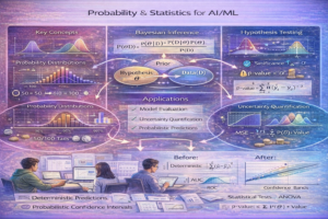
Probability & Statistics for AI/ML
Difficulty: Beginner | Time: 50-70 minutes | Key Concepts: Probability, Distributions, Statistics
Why Probability & Statistics Matter
machine learning is fundamentally about making predictions under uncertainty. Probability and statistics provide the tools to understand and manage that uncertainty.
1. Probability Fundamentals
What is Probability?
Probability is a number between 0 and 1 that represents the likelihood of an event occurring.
- P = 0: Event will never happen
- P = 0.5: Event has 50% chance
- P = 1: Event will definitely happen
Basic Probability Rules
Rule 1: Probability of Complement
P(NOT A) = 1 - P(A)

Example: If P(heads) = 0.5, then P(tails) = 1 - 0.5 = 0.5
Rule 2: Probability of Either Event
P(A OR B) = P(A) + P(B) - P(A AND B)

Example: P(red card OR face card) = P(red) + P(face) - P(red face card)
Rule 3: Conditional Probability
P(A|B) = P(A AND B) / P(B)

Read as: "Probability of A given B"

Example: P(rain|dark clouds) = P(rain AND dark clouds) / P(dark clouds)
2. Bayes’ Theorem (Most Important!)
The Formula
P(A|B) = P(B|A) × P(A) / P(B)
Real-World Example: Medical Test
You take a disease test. It's 99% accurate.
You test positive. What's the probability you have the disease?

Let D = has disease, T = tests positive
P(D|T) = P(T|D) × P(D) / P(T)

P(T|D) = 0.99 (if you have it, 99% chance test shows positive)
P(D) = 0.001 (1 in 1000 people have the disease)
P(T) = P(T|D)×P(D) + P(T|not D)×P(not D)
     = 0.99×0.001 + 0.01×0.999 = 0.01098

P(D|T) = (0.99 × 0.001) / 0.01098 ≈ 0.09 (only 9% chance!)
3. Probability Distributions
Normal Distribution (Gaussian)
The most important distribution in statistics. Most natural phenomena follow this bell curve.
- Defined by: mean (μ) and standard deviation (σ)
- 68% of data within 1σ of mean
- 95% of data within 2σ of mean
- 99.7% of data within 3σ of mean
Bernoulli Distribution
Binary outcomes: success (p) or failure (1-p)
Examples:
- Coin flip: P(heads) = 0.5
- Email spam filter: P(spam) = 0.05
- Click through rate: P(click) = 0.02
Uniform Distribution
All outcomes equally likely. Like a fair die (1/6 for each outcome).
4. Statistical Concepts
Mean (Average)
μ = (x₁ + x₂ + ... + xₙ) / n

Example: [1, 2, 3, 4, 5] → μ = 15/5 = 3
Variance & Standard Deviation
Variance (σ²): Average squared distance from mean
Standard Deviation (σ): Square root of variance = √variance

Example: [1, 3, 5]
μ = 3
Variance = ((1-3)² + (3-3)² + (5-3)²) / 3 = (4 + 0 + 4) / 3 ≈ 2.67
Std Dev = √2.67 ≈ 1.63
Correlation & Covariance
Covariance: How two variables change together
Correlation: Standardized covariance, ranges from -1 to 1
- Correlation = 1: Perfect positive relationship
- Correlation = 0: No relationship
- Correlation = -1: Perfect negative relationship
5. Hypothesis Testing
Null Hypothesis (H₀)
The assumption we’re testing (usually “no effect”)
Alternative Hypothesis (H₁)
What we believe if the null hypothesis is false
P-Value
Probability of observing our data if the null hypothesis is true
- P < 0.05: Usually considered "statistically significant"
- P > 0.05: Not enough evidence to reject null hypothesis
6. In Machine Learning Context
Classification Probabilities
Logistic Regression outputs probabilities:
P(class=1|x) = 1 / (1 + e^(-z))

Neural networks often output probabilities for each class
Maximum Likelihood Estimation
Training a model means finding parameters that maximize probability of observed data
Bayesian Machine Learning
Model posterior = likelihood × prior / evidence
P(θ|data) = P(data|θ) × P(θ) / P(data)
7. Python Examples
Probability Calculations
import numpy as np
from scipy import stats

# Normal distribution
dist = stats.norm(mu=0, sigma=1)
print(dist.pdf(0))    # Probability density at 0
print(dist.cdf(1))    # P(X <= 1) ≈ 0.84

# Bernoulli (coin flip)
coin = stats.bernoulli(p=0.5)
print(coin.pmf(1))    # P(heads) = 0.5

# Basic statistics
data = [1, 2, 3, 4, 5]
print(np.mean(data))   # 3.0
print(np.std(data))    # Standard deviation
print(np.var(data))    # Variance

# Correlation
x = [1, 2, 3, 4, 5]
y = [2, 4, 5, 4, 6]
correlation = np.corrcoef(x, y)[0, 1]
print(correlation)     # Correlation coefficient
8. Common Misconceptions
Misconception 1: High Probability = Will Happen
A 99% probability event still has 1% chance of not happening!
Misconception 2: Independent Events
Just because two things are correlated doesn’t mean one causes the other.
Misconception 3: Sample Represents Population
A small sample might not represent the entire population.
Key Takeaways
- Probability measures likelihood of events (0 to 1)
- Bayes’ theorem updates probabilities with new evidence
- Normal distribution is fundamental in statistics
- Mean and variance describe data distributions
- Correlation measures relationships between variables
- ML models learn probability distributions from data
Next: Learn Calculus
Next, learn Calculus for Machine Learning to understand optimization.
Resources
Continue Learning: Related Articles
Natural Language Processing: The Evolution from Rules to Neural Networks
The Journey of Natural Language Processing
Natural Language Processing (NLP) has undergone a remarkable transformation …
📖 5 min read
Create a Resume Parser with NLP: Complete Python Tutorial for Extracting Structured Data
Introduction to AI Resume Parsing
Resume parsing is a fundamental task in HR technology, powering applicant tracking sy…
📖 20 min read
AI Content Moderation Platforms: Perspective API vs Two Hat vs Azure Content Moderator vs Crisp Thinking
AI Content Moderation Platforms: Comparing Solutions for Online Safety 2025
User-generated content platforms face enorm…
📖 6 min read
Reinforcement Learning in Game AI: From Theory to Mastery
The Evolution of Game AI Through Reinforcement learning
Reinforcement learning (RL) has emerged as one of the most prom…
📖 5 min read
💡 Explore 80+ AI implementation guides on Harshith.org